In this blog post, you will learn several new skills and concepts related to image classification in Tensorflow.

• Tensorflow Datasets provide a convenient way for us to organize operations on our training, validation, and test data sets.
• Data augmentation allows us to create expanded versions of our data sets that allow models to learn patterns more robustly.
• Transfer learning allows us to use pre-trained models for new tasks.

Working on the coding portion of the Blog Post in Google Colab is strongly recommended. When training your model, enabling a GPU runtime (under Runtime -> Change Runtime Type) is likely to lead to significant speed benefits.

The Task

Can you teach a machine learning algorithm to distinguish between pictures of dogs and pictures of cats?

According to this helpful diagram below, one way to do this is to attend to the visible emotional range of the pet:

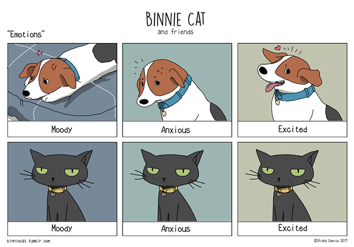
Unfortunately, using this method requires that we have access to multiple images of the same individual. We will consider a setting in which we have only one image for pet. Can we reliably distinguish between cats and dogs in this case?

Acknowledgment

Major parts of this Blog Post assignment, including several code chunks, are based on the TensorFlow Transfer Learning Tutorial. You may find that consulting this tutorial is helpful while completing this assignment, although this shouldn’t be necessary.

Start by making a code block in which you’ll hold your import statements. You can update this block as you go. For now, include

import os
from tensorflow.keras import utils 

Now, let’s access the data. We’ll use a sample data set provided by the TensorFlow team that contains labeled images of cats and dogs.

Paste and run the following code block.

# location of data
_URL = 'https://storage.googleapis.com/mledu-datasets/cats_and_dogs_filtered.zip'

# download the data and extract it
path_to_zip = utils.get_file('cats_and_dogs.zip', origin=_URL, extract=True)

# construct paths
PATH = os.path.join(os.path.dirname(path_to_zip), 'cats_and_dogs_filtered')

train_dir = os.path.join(PATH, 'train')
validation_dir = os.path.join(PATH, 'validation')

# parameters for datasets
BATCH_SIZE = 32
IMG_SIZE = (160, 160)

# construct train and validation datasets 
train_dataset = utils.image_dataset_from_directory(train_dir,
                                                   shuffle=True,
                                                   batch_size=BATCH_SIZE,
                                                   image_size=IMG_SIZE)

validation_dataset = utils.image_dataset_from_directory(validation_dir,
                                                        shuffle=True,
                                                        batch_size=BATCH_SIZE,
                                                        image_size=IMG_SIZE)

# construct the test dataset by taking every 5th observation out of the validation dataset
val_batches = tf.data.experimental.cardinality(validation_dataset)
test_dataset = validation_dataset.take(val_batches // 5)
validation_dataset = validation_dataset.skip(val_batches // 5)

By running this code, we have created TensorFlow Datasets for training, validation, and testing. You can think of a Dataset as a pipeline that feeds data to a machine learning model. We use data sets in cases in which it’s not necessarily practical to load all the data into memory.

In our case, we’ve used a special-purpose keras utility called image_dataset_from_directory to construct a Dataset. The most important argument is the first one, which says where the images are located. The shuffle argument says that, when retrieving data from this directory, the order should be randomized. The batch_size determines how many data points are gathered from the directory at once. Here, for example, each time we request some data we will get 32 images from each of the data sets. Finally, the image_size specifies the size of the input images, just like you’d expect.

Paste the following code into the next block. This is technical code related to rapidly reading data. If you’re interested in learning more about this kind of thing, you can take a look here.

AUTOTUNE = tf.data.AUTOTUNE

train_dataset = train_dataset.prefetch(buffer_size=AUTOTUNE)
validation_dataset = validation_dataset.prefetch(buffer_size=AUTOTUNE)
test_dataset = test_dataset.prefetch(buffer_size=AUTOTUNE)

Working with Datasets

You can get a piece of a data set using the take method; e.g. train_dataset.take(1) will retrieve one batch (32 images with labels) from the training data.

Let’s briefly explore our data set. Write a function to create a two-row visualization. In the first row, show three random pictures of cats. In the second row, show three random pictures of dogs. You can see some related code in the linked tutorial above, although you’ll need to make some modifications in order to separate cats and dogs by rows. A docstring is not required.

Check Label Frequencies

The following line of code will create an iterator called labels.

labels_iterator= train_dataset.unbatch().map(lambda image, label: label).as_numpy_iterator()

Compute the number of images in the training data with label 0 (corresponding to "cat") and label 1 (corresponding to "dog").

The baseline machine learning model is the model that always guesses the most frequent label. Briefly discuss how accurate the baseline model would be in our case.

We’ll treat this as the benchmark for improvement. Our models should do much better than baseline in order to be considered good data science achievements!

Create a tf.keras.Sequential model using some of the layers we’ve discussed in class. In each model, include at least two Conv2D layers, at least two MaxPooling2D layers, at least one Flatten layer, at least one Dense layer, and at least one Dropout layer. Train your model and plot the history of the accuracy on both the training and validation sets. Give your model the name model1.

To train a model on a Dataset, use syntax like this:

history = model1.fit(train_dataset, 
                     epochs=20, 
                     validation_data=validation

Here and in later parts of this assignment, training for 20 epochs with the Dataset settings described above should be sufficient.

You don’t have to show multiple models, but please do a few experiments to try to get the best validation accuracy you can. Briefly describe a few of the things you tried. Please make sure that you are able to consistently achieve at least 52% validation accuracy in this part (i.e. just a bit better than baseline).

1. In bold font, describe the validation accuracy of your model during training. You don’t have to be precise. For example, “the accuracy of my model stabilized between 65% and 70% during training.”
2. Then, compare that to the baseline. How much better did you do?
3. Overfitting can be observed when the training accuracy is much higher than the validation accuracy. Do you observe overfitting in model1?

Now we’re going to add some data augmentation layers to your model. Data augmentation refers to the practice of including modified copies of the same image in the training set. For example, a picture of a cat is still a picture of a cat even if we flip it upside down or rotate it 90 degrees. We can include such transformed versions of the image in our training process in order to help our model learn so-called invariant features of our input images.

1. First, create a tf.keras.layers.RandomFlip() layer. Make a plot of the original image and a few copies to which RandomFlip() has been applied. Make sure to check the documentation for this function!
2. Next, create a tf.keras.layers.RandomRotation() layer. Check the docs to learn more about the arguments accepted by this layer. Then, make a plot of both the original image and a few copies to which RandomRotation() has been applied.

Now, create a new tf.keras.models.Sequential model called model2 in which the first two layers are augmentation layers. Use a RandomFlip() layer and a RandomRotation() layer. Train your model, and visualize the training history.

Please make sure that you are able to consistently achieve at least 55% validation accuracy in this part. Scores of near 60% are possible.

Note: You might find that your model in this section performs a bit worse than the one before, even on the validation set. If so, just comment on it! That doesn’t mean there’s anything wrong with your approach. We’ll see improvements soon.

1. In bold font, describe the validation accuracy of your model during training.
2. Comment on this validation accuracy in comparison to the accuracy you were able to obtain with model1.
3. Comment again on overfitting. Do you observe overfitting in model2?

Sometimes, it can be helpful to make simple transformations to the input data. For example, in this case, the original data has pixels with RGB values between 0 and 255, but many models will train faster with RGB values normalized between 0 and 1, or possibly between -1 and 1. These are mathematically identical situations, since we can always just scale the weights. But if we handle the scaling prior to the training process, we can spend more of our training energy handling actual signal in the data and less energy having the weights adjust to the data scale.

The following code will create a preprocessing layer called preprocessor which you can slot into your model pipeline.

i = tf.keras.Input(shape=(160, 160, 3))
x = tf.keras.applications.mobilenet_v2.preprocess_input(i)
preprocessor = tf.keras.Model(inputs = [i], outputs = [x])

I suggest incorporating the preprocessor layer as the very first layer, before the data augmentation layers. Call the resulting model model3.

Now, train this model and visualize the training history. This time, please make sure that you are able to achieve at least 70% validation accuracy.

1. In bold font, describe the validation accuracy of your model during training.
2. Comment on this validation accuracy in comparison to the accuracy you were able to obtain with model1.
3. Comment again on overfitting. Do you observe overfitting in model3?

So far, we’ve been training models for distinguishing between cats and dogs from scratch. In some cases, however, someone might already have trained a model that does a related task, and might have learned some relevant patterns. For example, folks train machine learning models for a variety of image recognition tasks. Maybe we could use a pre-existing model for our task?

To do this, we need to first access a pre-existing “base model”, incorporate it into a full model for our current task, and then train that model.

Paste the following code in order to download MobileNetV2 and configure it as a layer that can be included in your model.

IMG_SHAPE = IMG_SIZE + (3,)
base_model = tf.keras.applications.MobileNetV2(input_shape=IMG_SHAPE,
                                               include_top=False,
                                               weights='imagenet')
base_model.trainable = False

i = tf.keras.Input(shape=IMG_SHAPE)
x = base_model(i, training = False)
base_model_layer = tf.keras.Model(inputs = [i], outputs = [x])

Now, create a model called model4 that uses MobileNetV2. For this, you should definitely use the following layers:

1. The preprocessor layer from Part §4.
2. The data augmentation layers from Part §3.
3. The base_model_layer constructed above.
4. A Dense(2) layer at the very end to actually perform the classification.

Between 3. and 4., you might want to place a small number of additional layers, like GlobalMaxPooling2D or possibly Dropout. You don’t need a lot though! Once you’ve constructed the model, check the model.summary() to see why – there is a LOT of complexity hidden in the base_model_layer. Show the summary and comment. How many parameters do we have to train in the model?

Finally, train your model for 20 epochs, and visualize the training history.

This time, please make sure that you are able to achieve at least 95% validation accuracy. That’s not a typo!

1. In bold font, describe the validation accuracy of your model during training.
2. Comment on this validation accuracy in comparison to the accuracy you were able to obtain with model4.
3. Comment again on overfitting. Do you observe overfitting in model4?

Feel free to mess around with various model structures and settings in order to get the best validation accuracy you can. Finally, evaluate the accuracy of your most performant model on the unseen test_dataset. How’d you do?

Turn your work into a tutorial Blog Post on the topic of image classification and transfer learning. Make sure to include all the code, summaries, and plots that you created. You might find it useful to refer to the Keras tutorial linked above, but your entire post should be in your own original words. Feel free to link your reader to any resources that you found helpful.

Please remember that you must meet all specifications in order to receive credit on the first submission!

Coding Problem

1. The visualization in Part 1 is implemented using a function and shows labeled images of cats in one row and labeled images of dogs in another row.
2. There are two visualizations in Part 3 showing the results of applying RandomFlip and RandomRotation to an example image.
3. Models 1, 2, 3, and 4 are logically constructed and obtain the required validation accuracy in each case:
   • Model 1 should obtain at least 52% validation accuracy.
   • Model 2 should obtain at least 55% validation accuracy.
   • Model 3 should obtain at least 70% validation accuracy.
   • Model 4 should obtain at least 95% validation accuracy.
4. The training history is shown for each of the four models, including the training and validation performance.
5. The most performant model is evaluated on the test data set.

Style and Documentation

1. Code throughout is written using minimal repetition and clean style.
2. Docstrings are not required in this Blog Post, but please make sure to include useful comments and detailed explanations for each of your code blocks.

Writing

1. The blog post is written in tutorial format, in engaging and clear English. Grammar and spelling errors are acceptable within reason.