January 18th, 2018
Draft Session Titles
Uh…what's data science?
An oversimplified categorization:
- Data science produces insights
- Machine learning produces predictions
- Artificial intelligence produces actions
(From David Robinson)
So, how do we get insights?
My Favorite Picture
My Favorite Picture

My Favorite Picture

My Favorite Picture

My Favorite Third Favorite Picture
 (Image credit: Hadley Wickham)
…

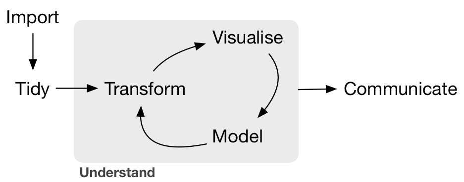
What we've done together already
- Import -> tidy -> transform
- Import -> tidy -> transform -> model
- Import -> tidy -> transform -> visualize
But….
Gameplan
- Work through an extended example of the (data-) scientific method.
- Learn key tools for building complex data pipelines from simple building blocks.
- Impress Patrick Stewart:

Warmup
Remember this?
Pull if you haven't already and fire up RStudio.
Exercise 0
- Look left.
- Look right.
- Pick a partner (groups of three are fine).
- Give them a friendly, professional smile.
- Maybe a handshake too.

Case Study, Part 1
- Explore the data
- Ask a question
- Form a hypothesis
A "basic" problem

- We'd like to investigate the listings that are driving that spike in April.
- First, we need to isolate them.
- Ideas?
Basic Trend Analysis
- Remove the seasonal (long term) and weekly (short term) trends, leaving the April bump.
- Separate out individual listings using k-means.
What we'd like to do

Fitting a Single Model
We'd like to fit a smoother to each listing to long-term trend. We can fit a single one like this:
model_data <- prices %>%       # extract a single listing's
    filter(listing_id == 5506) # worth of data

# fit a loess model, the span is a hyperparameter, a bit
# like lambda in LASSO
single_model <-  loess(price_per ~ as.numeric(date),
                       data = model_data,
                       span = .5)
Examining a Single Model
single_model %>% summary()
## Call:
## loess(formula = price_per ~ as.numeric(date), data = model_data,
##     span = 0.5)
##
## Number of Observations: 344
## Equivalent Number of Parameters: 6.32
## Residual Standard Error: 8.15
## Trace of smoother matrix: 6.95  (exact)
##
## Control settings:
##   span     :  0.5
##   degree   :  2
##   family   :  gaussian
##   surface  :  interpolate      cell = 0.2
##   normalize:  TRUE
##  parametric:  FALSE
## drop.square:  FALSE
Model Information the Tidy Way
model_preds <- broom::augment(single_model, model_data)
model_preds %>% head()
##   listing_id       date price_per  .fitted  .se.fit     .resid
## 1       5506 2017-09-05      72.5 73.73994 2.042531 -1.2399385
## 2       5506 2017-09-04      72.5 73.66160 1.984215 -1.1615956
## 3       5506 2017-09-03      72.5 73.58551 1.927151 -1.0855140
## 4       5506 2017-09-02      72.5 73.51158 1.871376 -1.0115812
## 5       5506 2017-09-01      72.5 73.43968 1.816931 -0.9396847
## 6       5506 2017-08-31      72.5 73.36971 1.763855 -0.8697121
Visualizing a Single Model
model_preds %>%
    ggplot(aes(x = date)) +
    geom_line(aes(y = price_per)) +
    geom_line(aes(y = .fitted), color = 'red')

How do we do this for multiple models?
model_container <- ????
for(id in unique(prices$listing_id)){
    model <- prices %>%
        filter(listing_id == id) %>%
        loess(price_per ~ as.numeric(date),
              data = .,
              span = .25)

    model_container %>% update(model) # ?????
    .
    .
    .
}
For loops…

A familiar loop
my_list <- list('To', 'boldly', 'go', 'where', 'no', 'man', 'has', 'gone', 'before')

length_list <- list()
i           <- 1
for(word in my_list){
    length_list[i] <- nchar(word)
    i              <- i + 1
}

length_list %>% unlist() # just for display
## [1] 2 6 2 5 2 3 3 4 6
A better way:
my_list <- list('To', 'boldly', 'go', 'where', 'no', 'man', 'has', 'gone', 'before')

length_list <- map(my_list, nchar) # or my_list %>% map(nchar)

length_list %>% unlist() # just for display
## [1] 2 6 2 5 2 3 3 4 6
purrr::map() applies a function (nchar) to each entry of the original list.
Map-Reduce
Use map to apply the same operation to a list of objects. Use reduce to combine them all together.
# product of the number of letters in each word
my_list %>%
    map(nchar) %>%
    reduce(`*`) # `*` is the product function: `*`(a,b) = a*b
## [1] 51840
Exercise
The directory exercise_data contains price data for each month. Use map + reduce to read it in and combine it as a single data set. You'll need read_csv and rbind.
Hint: start with list.files('exercise_data', full.names = T)
list.files('exercise_data', full.names = T) %>%
    map(read_csv) %>%
    reduce(rbind) %>%
    head() # just for display
## Parsed with column specification:
## cols(
##   listing_id = col_integer(),
##   date = col_date(format = ""),
##   price_per = col_double()
## )
## Parsed with column specification:
## cols(
##   listing_id = col_integer(),
##   date = col_date(format = ""),
##   price_per = col_double()
## )
## Parsed with column specification:
## cols(
##   listing_id = col_integer(),
##   date = col_date(format = ""),
##   price_per = col_double()
## )
## Parsed with column specification:
## cols(
##   listing_id = col_integer(),
##   date = col_date(format = ""),
##   price_per = col_double()
## )
## Parsed with column specification:
## cols(
##   listing_id = col_integer(),
##   date = col_date(format = ""),
##   price_per = col_double()
## )
## Parsed with column specification:
## cols(
##   listing_id = col_integer(),
##   date = col_date(format = ""),
##   price_per = col_double()
## )
## Parsed with column specification:
## cols(
##   listing_id = col_integer(),
##   date = col_date(format = ""),
##   price_per = col_double()
## )
## Parsed with column specification:
## cols(
##   listing_id = col_integer(),
##   date = col_date(format = ""),
##   price_per = col_double()
## )
## Parsed with column specification:
## cols(
##   listing_id = col_integer(),
##   date = col_date(format = ""),
##   price_per = col_double()
## )
## Parsed with column specification:
## cols(
##   listing_id = col_integer(),
##   date = col_date(format = ""),
##   price_per = col_double()
## )
## Parsed with column specification:
## cols(
##   listing_id = col_integer(),
##   date = col_date(format = ""),
##   price_per = col_double()
## )
## Parsed with column specification:
## cols(
##   listing_id = col_integer(),
##   date = col_date(format = ""),
##   price_per = col_double()
## )
## # A tibble: 6 x 3
##   listing_id       date price_per
##        <int>     <date>     <dbl>
## 1    3075044 2017-04-30      32.5
## 2    3075044 2017-04-29      37.5
## 3    3075044 2017-04-28      37.5
## 4    3075044 2017-04-27      32.5
## 5    3075044 2017-04-26      32.5
## 6    3075044 2017-04-25      32.5
Fundamental Pattern
Use lists of data frames (and data frames of lists) to organize your work.
Why?
Data frames are the fundamental unit of data science.
Usually their columns are atomic vectors of integers, doubles, dates, characters, or booleans. E.g.
## # A tibble: 6 x 3
##   listing_id       date price_per
##        <int>     <date>     <dbl>
## 1    3075044 2017-08-22      32.5
## 2    3075044 2017-08-21      32.5
## 3    3075044 2017-08-20      32.5
## 4    3075044 2017-08-19      37.5
## 5    3075044 2017-08-18      37.5
## 6    3075044 2017-08-17      32.5
But this is somewhat inflexible. What about more complex objects? Lists can hold anything…
Well if lists are so great…

That's a good idea!
prices_nested <- prices %>%
    tidyr::nest(-listing_id)

# view the data types of the columns
map(prices_nested, class) %>% unlist()
## listing_id       data
##  "integer"     "list"
Ew.

Actually…
prices_nested %>% head()
## # A tibble: 6 x 2
##   listing_id               data
##        <int>             <list>
## 1    3075044 <tibble [359 x 2]>
## 2       6976 <tibble [319 x 2]>
## 3    7651065 <tibble [334 x 2]>
## 4    5706985 <tibble [344 x 2]>
## 5    2843445 <tibble [365 x 2]>
## 6     753446 <tibble [347 x 2]>
WELP

Just checking
prices_nested$data[[1]] # get the first item of the list
## # A tibble: 359 x 2
##          date price_per
##        <date>     <dbl>
##  1 2017-08-22      32.5
##  2 2017-08-21      32.5
##  3 2017-08-20      32.5
##  4 2017-08-19      37.5
##  5 2017-08-18      37.5
##  6 2017-08-17      32.5
##  7 2017-08-16      32.5
##  8 2017-08-15      32.5
##  9 2017-08-14      32.5
## 10 2017-08-13      32.5
## # ... with 349 more rows
We were here:
Now we're here:

Exercise
Use map to extract a list of lengths of each data frame in prices_nested$data
lengths <- map(prices_nested$data, nrow)
lengths %>% unlist() %>% head() # for display only
## [1] 359 319 334 344 365 347
Exercise
Write a function that extracts the largest price (per person) from a data frame.
get_biggest_price <- function(data){
    data$price_per %>% max(na.rm = T)
}
Now map to extract the largest price in each data frame in prices_nested$data:
biggest_prices <- map(prices_nested$data, get_biggest_price)
biggest_prices %>% head() %>% unlist()
## [1] 37.50000 32.50000 39.50000 66.66667 37.50000 34.50000
Exercise
Now do the same thing, but assign the result to a new list column of prices_nested. Don't forget what you learned in Session 2!
prices_nested %>%
    mutate(highest_price = map(data, get_biggest_price))
## # A tibble: 5 x 3
##   listing_id               data highest_price
##        <int>             <list>        <list>
## 1    3075044 <tibble [359 x 2]>     <dbl [1]>
## 2       6976 <tibble [319 x 2]>     <dbl [1]>
## 3    7651065 <tibble [334 x 2]>     <dbl [1]>
## 4    5706985 <tibble [344 x 2]>     <dbl [1]>
## 5    2843445 <tibble [365 x 2]>     <dbl [1]>
Exercise
Now do the same thing, but assign the result to a new list column of prices_nested.
prices_nested %>%
    mutate(highest_price = map_dbl(data, get_biggest_price))
## # A tibble: 5 x 3
##   listing_id               data highest_price
##        <int>             <list>         <dbl>
## 1    3075044 <tibble [359 x 2]>      37.50000
## 2       6976 <tibble [319 x 2]>      32.50000
## 3    7651065 <tibble [334 x 2]>      39.50000
## 4    5706985 <tibble [344 x 2]>      66.66667
## 5    2843445 <tibble [365 x 2]>      37.50000
Summing Up
We know how to:
- Nest a data frame, creating a list of data frames.
- Use
mapto apply a function to every element of a list. - Apply a model function to an individual data frame (from Session 3).
Looks like it's time for…
Case Study, Part 2
- Fit many models
- Learn from results
- Ask new questions
We were here:
Then we did this:

Now we're here:


In code
my_loess <- function(data, span){
    loess(price_per ~ as.numeric(date),
    data = data,
    span = span)
}

prices_nested <- prices %>%
    nest(-listing_id)

prices_modeled <- prices_nested %>%
    mutate(model = map(data, my_loess, span = .25))

prices_with_preds <- prices_modeled %>%
    mutate(preds = map2(model, data, augment))

prices_unnested <- prices_with_preds %>%
    unnest(preds)
More concise with %>%
my_loess <- function(data, span){
    loess(price_per ~ as.numeric(date),
    data = data,
    span = span)
}

prices_unnested <- prices %>%
    nest(-listing_id) %>%
    mutate(model = map(data, my_loess, span = .25),
           preds = map2(model, data, augment)) %>%
    unnest(preds)
Even more concise
A little syntactic sugar (reference)
prices_unnested <- prices %>%
    nest(-listing_id) %>%
    mutate(model = map(data, ~loess(price_per ~ as.numeric(date), data = ., span = .25)),
           preds = map2(model, data, augment)) %>%
    unnest(preds)

Thousands of models, four lines
prices_unnested <- prices %>%
    nest(-listing_id) %>%
    mutate(model = map(data, ~loess(price_per ~ as.numeric(date), data = ., span = .25)),
           preds = map2(model, data, augment)) %>%
    unnest(preds)
Four nontrivial lines:
- Nest the data…
- …Fit a collection of the models to the data (map)…
- …Augment the data with the model predictions…
- …Unnest the data…
…and now we're ready to explore the results.
The Data Science Pipeline
Break Time
Reminder: What we're up to
- Remove the seasonal (long term) and weekly (short term) trends, leaving the April bump.
- Separate out individual listings using k-means.

Case Study Part 3
- Fit many models
- Learn from results
- Ask new questions
Closing Out
My Favorite Third Favorite Picture
Takeaways
- Data science is nonlinear – learn to love the cycle.
- Modeling isn't always the final step – sometimes it's a cleaning step for the analysis you really want to do.
- The
tidyverseset of packages gives you a powerful toolbox for accomplishing complex tasks with simple code.
Closing Thought

Reference
Learn More About Our Packages
More on the Tidyverse
- R For Data Science is a book by Garrett Grolemund and Hadley Wickham that goes deep into a complete suite of tools for the data science pipeline.
Other "Advanced Topics in Data Science"
- Automating long data science pipelines with GNU
make. - Literate programming with RMarkdown. These slides, as well as the "pretty" lecture notes, were made in
R! - Interactive data applications with Shiny
- Develop your own
Rpackages. - Structure of the
Rlanguage – check out Advanced R.